
A stability lobe diagram (SLD) maps spindle speed against axial depth of cut to reveal the RPM pockets where regenerative chatter is unlikely, letting you push material removal rate without the tool singing. Its real value shows up when you use it to select spindle speeds inside a lobe peak instead of defaulting to a conservative depth. The catch: an SLD is only as good as the machine, holder, and tool combination it was measured or calculated for, so every diagram needs a cutting-test check before you trust it in production.
TL;DR:
- The accuracy of a stability lobe diagram depends on precise FRF measurements taken directly from the actual tool, holder, and machine setup.
- Shifts in tool wear, fixture clamping, or structural changes can significantly alter the FRF, requiring re-measurement and revalidation of the diagram.
- Modern fast FRF-based computation methods provide similar accuracy to traditional analytical models but are practical for real-time updates.
- Confirming a lobe peak with a short validation cut and logging results against specific tool states improves reliability during production.
- Routine re-measurement and validation are essential because the static SLD only reflects the system at one point in its tool life, not the entire process lifespan.
Table of Contents
- What Chatter Stability Lobes Actually Represent
- Altintas–Budak Theory and Fast FRF-Based Prediction
- Measuring FRF and Extracting Modal Parameters on the Shop Floor
- Mapping Lobes Fast: In-Process Testing and Chatter Detection
- Turning Lobe Data Into a Production-Ready Speed
- Why Stability Lobes Sometimes Fail to Predict Reality
- How Availzye Machinist Pro Supports the SLD Workflow
- Your Stability Lobe Checklist Before the Next Deep Cut
- The Overlooked Trade-Off in Stability Lobe Tuning
- Get Your Stability Lobe Workflow Running This Week
- Sources
What Chatter Stability Lobes Actually Represent
A stability lobe diagram is the graphical answer to one question: at this spindle speed, how deep can you cut before the tool starts vibrating uncontrollably? The x-axis runs spindle speed, the y-axis runs axial depth of cut, and a scalloped boundary curve separates the stable region below from the chatter zone above. That scalloped shape is not decoration. It comes directly from the physics of regenerative chatter.
Regenerative chatter happens because a cutting edge never meets a perfectly flat surface. Each tooth leaves a wavy imprint from the vibration of the tooth before it, so the next tooth cuts a slightly varying chip thickness. That variation feeds force fluctuations back into the structure, and if the timing lines up wrong relative to the tooth-passing frequency, the vibration grows instead of damping out. It is a feedback loop between the surface texture from one revolution and the cut on the next.
The lobes exist because that feedback isn't equally destructive at every speed. At certain spindle speeds, the phase relationship between the structural vibration and the tooth-passing frequency causes partial cancellation, which raises the depth of cut a machine can tolerate before chatter onset. Those favorable speeds cluster around integer fractions of the dominant natural frequency, and each cluster forms one lobe. Between lobes, the phase relationship works against you, and the stable depth collapses toward a floor value engineers call b_lim,min.
Reading an SLD comes down to three landmarks:
- The stable region below the curve, where any axial depth is chatter-free at that spindle speed.
- The unstable region above the curve, where the same depth would trigger chatter at that speed.
- Lobe peaks and b_lim,min, the sweet spots and the floor value that tell you how much headroom a given RPM offers.
Shift the spindle speed just a few hundred RPM and you can move from a lobe peak, where three times the depth is stable, to a valley where the tool chatters immediately. That sensitivity is why guessing at speeds costs shops real material removal rate they never recover.
Altintas–Budak Theory and Fast FRF-Based Prediction
The analytical backbone for nearly every modern SLD calculator traces back to Altintas–Budak stability theory, which derives the chatter boundary directly from the machine-tool-workpiece frequency response function. Instead of running dozens of physical cuts, you feed in the dynamic stiffness of the system and the theory returns the axial depth limit at every spindle speed.
The math hinges on the oriented FRF, often written as Λ, which combines the directional cutting force coefficients with the measured frequency response to produce the critical depth of cut at each chatter frequency. Once you have Λ, the lobe centers fall out of a straightforward relationship: Ω_k = 60·f_c/(N·(k+1)), where f_c is the chatter frequency, N is the tooth count, and k is the lobe number (0, 1, 2, and so on). Higher-order lobes (larger k) sit closer together and shrink in width, which is why high-speed spindles chase the first two or three lobes rather than trying to exploit the tenth one.
Three modal parameters drive the whole calculation:
- Natural frequency (f_n), which sets where the dominant chatter tendency sits.
- Modal stiffness (k), which governs how much force it takes to deflect the structure.
- Damping ratio (ζ), which determines how quickly vibration energy dissipates and how deep the stable pockets can get.
Here's the trade-off that matters on a shop floor: full analytical stability solutions used to take meaningful computation time per tool-holder combination, which made them impractical to rerun every time a setup changed. Fast prediction methods built on measured FRF data or fitted modal parameters closed that gap and are supported by Engineering Simulation Software & Tools | Jewlz Technologies. Published comparisons show FRF and modal-parameter-based SLD prediction matching classical analytical results in accuracy while computing 2 to 3 orders of magnitude faster. That speed difference is what makes it realistic to recompute an SLD every time you swap a holder instead of once per quarter.
Pro Tip: If your calculator supports direct FRF import instead of requiring hand-fit modal parameters, use it. Curve-fitting introduces its own error, and skipping that step keeps the b_lim curve closer to what you'll actually see at the spindle.
Measuring FRF and Extracting Modal Parameters on the Shop Floor
Getting a usable stability lobe diagram starts with a frequency response function measurement, and that means putting real instrumentation on the actual tool-holder-spindle assembly you plan to run. Skip this step or borrow numbers from a similar setup, and the diagram you generate describes a machine that doesn't exist.
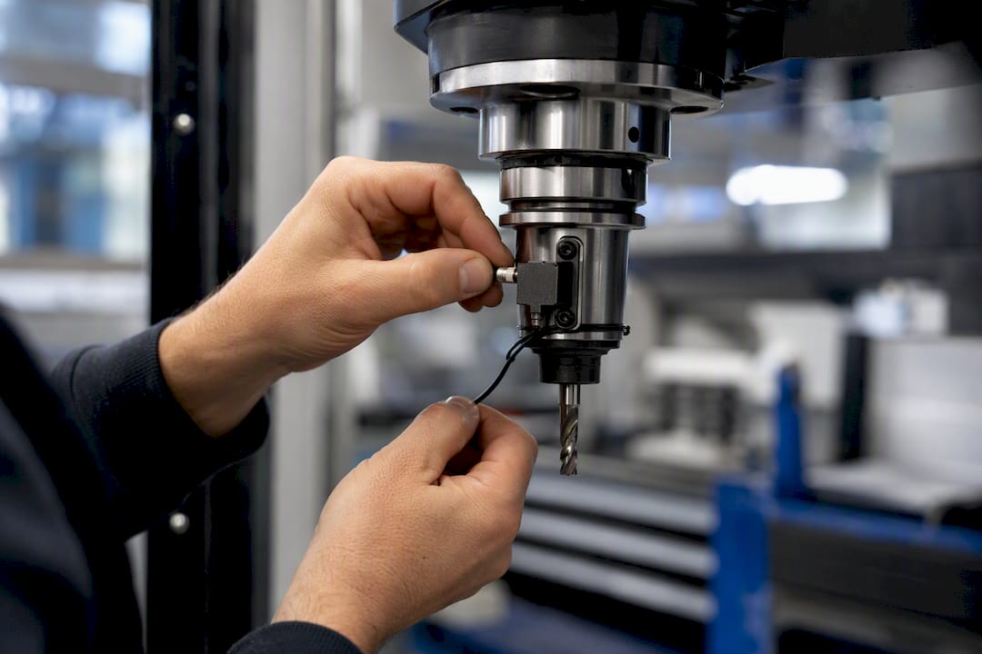
The standard measurement rig uses an instrumented impact hammer to excite the tool tip and an accelerometer, often mounted near the same point or on the spindle housing, to capture the resulting vibration response. Shops running spindles with active magnetic bearings can sometimes pull modal data directly from the AMB sensors already built into the spindle, skipping the external hardware entirely. Either way, you're measuring how the structure responds across a frequency sweep, not just at one tap.
The workflow itself follows a repeatable sequence:
- Strike the tool tip with the impact hammer at the point closest to where cutting forces will act, usually the free end of the tool.
- Record the force and acceleration signals simultaneously with a data acquisition system sampling fast enough to capture the frequencies of interest, typically well above the expected chatter frequency.
- Convert to the frequency domain with an FFT and divide acceleration by force to get the raw FRF.
- Check the coherence function across the frequency range; low coherence at any frequency means noise or a bad hit, and that data point should be discarded.
- Curve-fit the FRF using single-degree-of-freedom or multi-mode fitting to extract f_n, k, and ζ for each dominant mode.
The pitfalls cluster around variability you don't see until the numbers come back wrong. Toolholder clamping force changes the effective stiffness at the joint, so two identical tools in two different collets can produce meaningfully different FRFs. Bolted or shrink-fit joints add their own damping and stiffness that a purely analytical model of the tool and spindle will miss entirely, which is one reason modal-parameter extraction accuracy drives so much of overall SLD accuracy. Run the impact test two or three times and compare the resulting curves before trusting any single measurement; a repeatable FRF is the first sign your data is clean.
Mapping Lobes Fast: In-Process Testing and Chatter Detection
Full FRF measurement plus analytical computation gets you a theoretical diagram. Confirming it, or building one experimentally when instrumentation is limited, means cutting metal and watching how the process behaves in real time.
The classical experimental approach uses inclined-slot tests: you cut a slot at a gradually increasing depth while holding spindle speed constant, then watch for the axial depth where chatter marks appear on the surface. Running that test at several different spindle speeds and connecting the transition points builds an empirical stability boundary, point by point.
That grid approach works but eats machine time. Faster methods collapse the process into fewer passes:
- Ramp spindle speed continuously during a single cut at fixed depth, letting the process sweep through multiple lobes in one pass and revealing where chatter onset occurs relative to RPM.
- Ramp depth of cut continuously at a fixed or slowly varying spindle speed to find the instantaneous stability limit without stopping between tests.
- Combine both continuous variations in a coordinated in-process test, which maps the stability boundary substantially faster than a traditional point-by-point grid.
None of that works without a reliable way to catch chatter onset the instant it happens, which is where online detection algorithms earn their keep. Poincaré map analysis samples the vibration signal once per tooth period and looks for the signal collapsing to a single point (stable) versus scattering across multiple points (chatter). Time-domain indicators track rising vibration amplitude or a shift in dominant frequency away from the tooth-passing rate, both of which flag instability before it shows up as visible chatter marks. Microphone-based and accelerometer-based detection criteria can feed straight into CNC control logic, logging the exact RPM and depth where the transition occurred without an operator standing over the machine listening for trouble.
Turning Lobe Data Into a Production-Ready Speed
An SLD only pays off once it changes what RPM and depth actually show up in a program. That means treating the diagram as a shortlist of candidates, not a final answer.
Start by identifying two or three lobe peaks that sit within your spindle's usable range, then cross-check each candidate RPM against the tool manufacturer's recommended cutting speed for that material and tool geometry. A lobe peak that lands well outside the recommended surface speed for the insert or coating will chew through tool life even while the SLD shows the cut as stable. The workable operating point sits at the intersection of a lobe peak and a speed the tool can actually survive.
Validation before committing a lobe-tuned speed to a production job should cover the whole assembled system, not just spindle RPM:
- Toolholder clamping, since collet wear or an underclamped shrink fit shifts the FRF you measured earlier.
- Overhang length, because a longer stickout drops the natural frequency and moves your lobe centers.
- Radial immersion and coolant delivery, both of which affect cutting force and, indirectly, stability at the margins.
- A short validation cut with surface inspection, checking for chatter marks under magnification before running the full depth.
- Accelerometer monitoring during the first production parts, catching marginal instability that a visual check alone would miss.
Practical guidance from experienced machinists on lobe tuning pushes shops away from a habit of over-conservatism: defaulting to shallow depths at safe-sounding round-number speeds wastes the lobe structure entirely. Deliberately riding a validated peak, once you've confirmed it holds, is where the material removal gains actually show up.
Pro Tip: Log every validation cut result, including the ones that failed, in a job tracker tied to the specific tool and holder combination. A lobe peak that worked with a fresh insert can shift as the tool wears, and a written record beats trying to remember which RPM caused trouble three jobs ago.
Scale gradually. Move from validation cuts to short production runs before committing an entire job to a newly tuned speed, and build in a periodic re-check as tools accumulate wear.
Why Stability Lobes Sometimes Fail to Predict Reality
Stability lobe theory assumes a linear, time-invariant system, and real machining environments violate that assumption more often than most SLD users expect. When a lobe-tuned RPM still chatters, the cause usually falls into one of a few categories:
- Mode coupling, a different instability mechanism entirely, where vibration in two structural directions couples together regardless of tooth-passing frequency. Mode-coupling chatter doesn't respond to RPM tuning at all; it needs structural fixes like added damping, a stiffer holder, or a tuned mass damper.
- Process damping at low spindle speeds, where the clearance face of the tool interacts with the wavy surface in ways the standard regenerative model ignores, often making the actual stable depth larger than the classical SLD predicts.
- Nonlinear force behavior at very shallow or very deep cuts, where the linearized cutting force model the SLD relies on starts to break down.
Tool wear adds a slower-moving complication. As a cutting edge wears, cutting force coefficients shift, and the effective stiffness and damping of the system change with it. An SLD computed for a fresh insert can drift out of alignment by the time that same tool is 70% through its life, which is part of why time-dependent stability models that track wear progression are gaining ground in production environments that can't afford surprise chatter on hour six of a long run.
How Availzye Machinist Pro Supports the SLD Workflow
Availzyemachinistpro's Chatter Prediction calculator accepts FRF or fitted modal parameters directly, so the modal data you pull from an impact test on the shop floor turns into a usable stability lobe diagram without a separate analysis package.
A typical loop looks like this:
- Import modal parameters (f_n, k, ζ) or raw FRF data from your measurement session.
- Generate the SLD and identify candidate lobe peaks against your spindle's RPM range.
- Cross-check candidate speeds using the platform's Feeds & Speeds and Tool Deflection calculators to confirm the cut holds up structurally at depth.
- Run validation cuts, then log results, tool wear state, and holder configuration in the Job Tracker so the next programmer inherits real data instead of guesswork.
- Track re-validation intervals through the Maintenance Tracker as tools and spindle bearings age.
That loop keeps the SLD tied to the actual assembly cutting the part, not a spreadsheet from six months ago.
Your Stability Lobe Checklist Before the Next Deep Cut
An SLD tells you where regenerative chatter is unlikely across spindle speed and depth, but it describes one specific machine, holder, and tool combination. Change any of those and the diagram needs a recheck.
Before trusting a lobe-tuned speed in production: measure the FRF on the actual assembly, compute or import the SLD, validate at your candidate RPM with a short test cut, monitor for chatter as the tool wears, and log every result against that specific tool and holder pairing.
The Overlooked Trade-Off in Stability Lobe Tuning
Most engineering writing on stability lobe diagrams treats the analytical calculation as the hard part and validation as an afterthought. That gets the emphasis backward. The math behind Altintas–Budak theory is well established and, with fast FRF-based methods, cheap to run repeatedly. The part shops actually get wrong is treating a computed or even a measured SLD as a fixed law rather than a snapshot of one assembly at one point in its tool life.
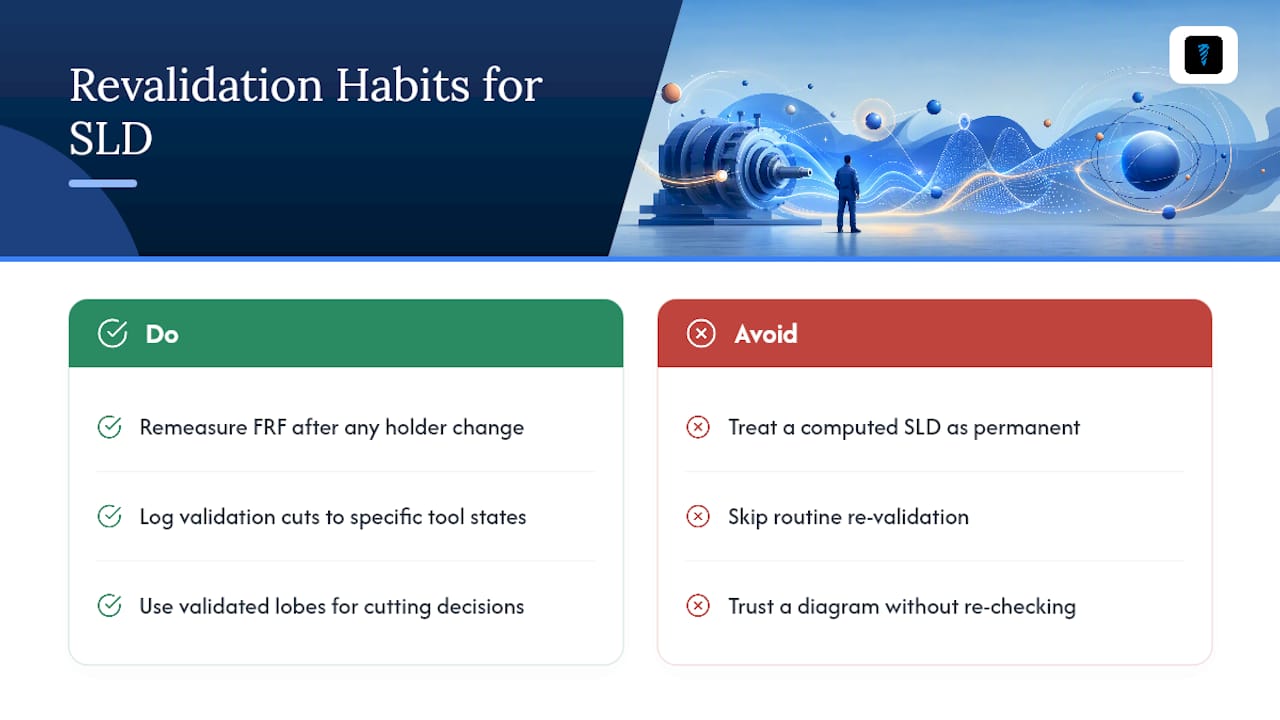
The conventional advice to "stay conservative" undersells what a validated lobe peak can do for material removal rate, and the opposite advice, trusting a diagram indefinitely without re-checking it, ignores how much a worn edge or a swapped holder shifts the whole curve. Both failure modes come from skipping the same step: routine re-validation.
If you take one thing from this, prioritize building the habit of remeasuring FRF after any holder change and logging validation cuts against specific tool states, not just building a bigger library of theoretical diagrams. The lobe math has matured. Shop discipline around when to trust it hasn't caught up.
— Availzye
Get Your Stability Lobe Workflow Running This Week
Availzyemachinistpro turns the SLD process into something you can run between setups instead of scheduling as a special project. Where a standalone analytical package leaves you exporting modal data and reformatting spreadsheets, the Chatter Prediction calculator sits inside the same platform as your feeds, speeds, and tool deflection math, so a validated RPM feeds straight into the rest of your programming without re-entering numbers.

That matters most for shops juggling multiple holders and tool lengths across a week's jobs, where remeasuring by hand every time a setup changes is the step that gets skipped under deadline pressure. Availzyemachinistpro's Job Tracker holds the validation history for each tool and holder combination, so the next programmer sees what already worked instead of starting from a conservative guess. Pair that with the G-code generator to move a validated speed and depth straight into a program, and the loop from measurement to cutting metal shrinks from days to a single shift. Start the 7-day free trial and run your next lobe-tuning pass through the full workflow before your next production job goes out the door.
Sources
- Analytical stability prediction and automated calculators (MDPI)
- Using stability lobe diagrams to control chatter (CTE Magazine)
- Fast prediction of chatter stability lobe diagram using FRF or modal parameters (Int J Adv Manuf Technol, 2017)
- Chatter stability fundamentals and measurement considerations (MTRC/UTK)