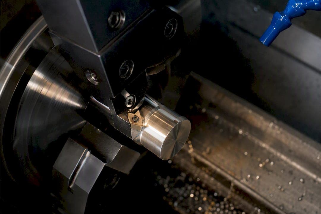
Taylor's tool life equation is V·Tⁿ = C, rearranged to solve for life as T = (C/V)^(1/n). V is cutting speed, T is tool life in minutes, and C and n are empirical constants specific to a tool and workpiece pairing. Plug in a speed, and you get a life prediction in minutes, no more complicated than that.
TL;DR:
- Small increases in cutting speed can significantly reduce tool life, especially with tools having a low n value, such as high-speed steel.
- Validating C and n constants through actual shop testing provides more reliable predictions than relying on textbook values or ranges.
- Extending the basic Taylor model to include feed rate, depth of cut, or coolant effects improves accuracy, but requires additional data and experimentation.
- Regular measurement of flank wear and logging it against predicted life helps calibrate and maintain accurate tool life estimations.
- Using software tools that store derived constants and automate calculations can streamline multiple tool management and improve prediction reliability.
Table of Contents
- The Taylor Tool Life Equation Explained Symbol by Symbol
- Typical n and C Values for Common Tool Materials
- How to Calculate Tool Life With Worked Examples
- How to Determine C and n for Your Own Tooling
- Where the Basic Taylor Equation Falls Short
- Checking Tool Life on the Shop Floor
- How Shop Software Applies Taylor's Equation in Practice
- Why Taylor's Equation Still Matters a Century Later
- Log Your Tool Life Data Instead of Guessing at Constants
- Sources
The Taylor Tool Life Equation Explained Symbol by Symbol
Every term in V·Tⁿ = C carries a specific job. Get the units wrong and the whole calculation falls apart, which happens more often than most machinists admit.
- V is cutting speed, typically in meters per minute (m/min) or surface feet per minute (SFM).
- T is tool life, almost always expressed in minutes to failure at the chosen wear endpoint.
- n is the Taylor exponent, a unitless number describing how sharply life reacts to speed changes.
- C is the cutting speed that would produce exactly one minute of tool life. It is not a physical speed you'd ever run.
To solve for life at a known speed, rearrange to T = (C/V)^(1/n). To solve for the speed that hits a target life, flip it again: V = C/(T^n). Both directions use the same three known values and one unknown, which is why the Taylor Tool Life Simulator from NovaSolver frames the whole relationship as one algebraic rearrangement rather than two separate formulas. Physically, n governs sensitivity to speed. A small n means life crashes fast when speed climbs even slightly. C sets the baseline: a higher C means the tool tolerates faster cutting before wearing out.
Typical n and C Values for Common Tool Materials
Textbook constants are starting points, not guarantees. Every real value has to be validated against your own machine, coolant, and workpiece batch before you trust it in production.
- High-speed steel (HSS): n typically runs 0.1 to 0.2, meaning life is highly sensitive to speed increases.
- Carbide: n typically runs 0.2 to 0.4, tolerating faster speeds before life collapses.
- Ceramics: n tends to run higher still, which is part of why ceramic inserts hold up at aggressive speeds in hardened steel work.
These ranges come from the Tool Life Predictor at AI CNC, which stresses that C and n must be derived experimentally for your specific tool, coating, and material combination. A textbook n of 0.25 for carbide on mild steel tells you nothing reliable about that same carbide grade running against a tougher alloy with a different coolant. Treat published ranges as a sanity check on your own data, not a substitute for it.
Sensitivity example: for a tool with n = 0.25, a 10% increase in cutting speed drops tool life to roughly 68% of its original value, according to sensitivity modeling from NovaSolver. That single relationship explains why shaving a few minutes off cycle time by pushing speed can quietly double your tool consumption rate.

How to Calculate Tool Life With Worked Examples
Two problems cover the two directions you'll actually use on the shop floor: solving for life, and solving for the speed that hits a target life.
- Solve for T. A carbide tool has C = 350 (m/min at 1 minute life) and n = 0.25. You're cutting at V = 120 m/min. T = (350/120)^(1/0.25) = (2.917)^4 ≈ 72.3 minutes. If your cycle time per part is 1.2 minutes, that tool edge is good for roughly 60 parts before it hits the wear endpoint.
- Solve for V. You need a target life of T = 45 minutes on that same tool (C = 350, n = 0.25). Rearranged: V = C/(T^n) = 350/(45^0.25) = 350/2.590 ≈ 135.1 m/min. Push past that speed and you're trading tool life for cycle time, whether or not that's the intended trade.
| Starting n | Speed increase | Resulting life (% of original) |
|---|---|---|
| 0.1 to 0.2 (typical HSS) | +10% | roughly 68% of original life |
| 0.2 to 0.4 (typical carbide) | +10% | ≈ 75% of original life |
That table is the whole argument for choosing carbide over HSS in speed-sensitive operations, and for treating small speed overrides on the shop floor as something worth logging, not ignoring. If you're dialing in feeds and speeds for a new job, this sensitivity gap should influence how much margin you build into your target speed.
How to Determine C and n for Your Own Tooling
Published constants describe someone else's machine, coolant, and material lot. Deriving your own C and n takes a handful of test cuts and a bit of log math, and it's worth doing for any tool you run in volume.
- Pick four or five cutting speeds spanning your realistic operating range, keeping feed and depth of cut fixed across all runs.
- Define one clear wear endpoint in advance (commonly 0.3 mm flank wear) and apply it consistently to every test.
- Log each run: speed, time to endpoint, feed, depth, coolant type, and machine.
- Take the log of both V and T for each data point, then run a linear regression. The slope of that line is negative 1/n; the intercept, once converted back, gives you C.
- Repeat at least one speed to check run-to-run variation before trusting the fit.
This log-linear extraction method mirrors what the Tool Life Predictor tool recommends for practitioners deriving shop-specific constants rather than relying on catalog numbers.
Pro Tip: Retest C and n any time you change coating, coolant chemistry, or workholding setup. A constant derived on a dry cut won't hold once you switch to flood coolant, even on the same tool and material.
Where the Basic Taylor Equation Falls Short
The original V·Tⁿ = C only accounts for cutting speed. It says nothing about feed rate, depth of cut, machine rigidity, coolant delivery, or tool runout, all of which move real tool life independently of speed.
- Feed rate and depth of cut both affect chip load and heat generation, neither of which the basic equation captures.
- Machine condition (spindle runout, worn bearings) can shorten life regardless of what V and T predict.
- Coolant type and delivery pressure change the thermal picture enough to shift C meaningfully.
Practitioners handle this by extending the model to V·Tⁿ·f^a·d^b = C, where f is feed, d is depth of cut, and a and b are additional exponents found experimentally, a form documented in the tool wear literature on Wikipedia. Full re-testing for every variable combination is expensive, so most shops apply simple correction factors for known deviations and reserve full re-derivation for major process changes, like a new coating or a different coolant family entirely.
Checking Tool Life on the Shop Floor
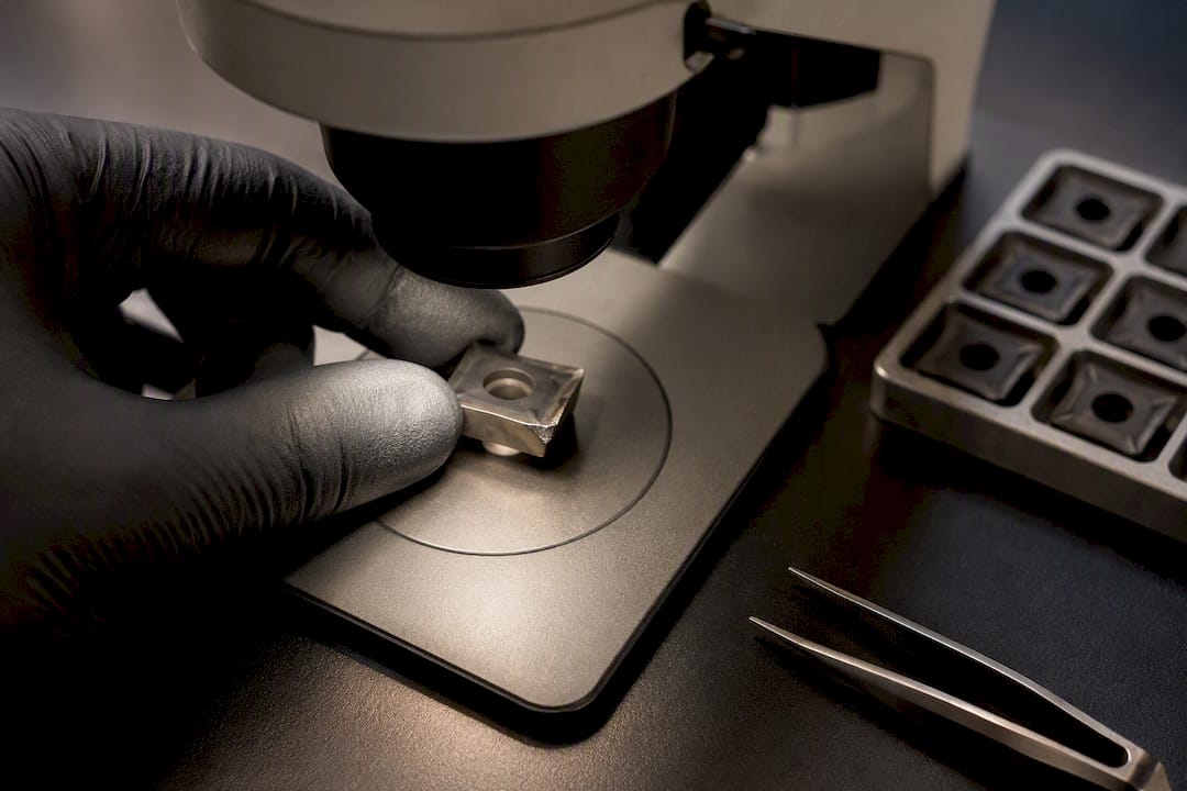
Predicted life from the equation is a planning number. What actually decides when a tool comes out is direct inspection against a defined wear threshold.
- Flank wear (VB) is the standard endpoint, commonly set around 0.3 mm before replacement.
- Crater wear and built-up edge (BUE) signal thermal or chip-evacuation problems even when flank wear looks fine.
- Surface finish drift and size drift on the part itself often catch wear before a visual inspection does.
Converting predicted minutes into a replacement schedule just means dividing life by your per-part cycle time, checked against surface finish measurements during a pilot run. The predictive maintenance approach many shops use for machines applies just as well to tooling: run a pilot batch, monitor actual wear against the predicted curve, and adjust the schedule before the deviation costs you scrapped parts.
Pro Tip: Don't wait for a tool to fail catastrophically to calibrate your model. Pull a tool at 80% of predicted life once per batch and measure actual flank wear. That single data point tells you fast whether your C and n still hold.
How Shop Software Applies Taylor's Equation in Practice
Running this math by hand for every job works fine for a classroom problem set. It gets tedious fast once you're managing a tool crib with dozens of active tool and material combinations.
- A built-in T↔V solver handles the algebra both directions, with unit conversion between SFM and m/min handled automatically.
- Parts-per-edge outputs translate a life prediction directly into a replacement count against your actual cycle time.
- Sensitivity charts visualize how a given n reacts to speed changes, the same relationship shown in the +10% examples above.
Availzye Machinist Pro's calculator suite includes a Taylor solver alongside its Feeds & Speeds tools, paired with a Tool Crib module that logs measured tool life against inventory. When a validation run produces a new C or n for a specific tool and material, that figure gets attached to the tool record instead of living in a separate spreadsheet, similar in spirit to how model-tracking systems in other trades prevent techs from grabbing the wrong part for a job. Storing constants next to inventory data, rather than treating them as universal, is the discipline the equation actually rewards.
Why Taylor's Equation Still Matters a Century Later
Taylor's equation is best treated as an economics tool, not a failure predictor. It tells you the trade-off between cutting faster and changing tools more often, which is exactly the calculation a shop needs to price a job correctly. Frederick Taylor's original relationship dates to 1907, and it has survived because that trade-off never went away.
If you're teaching this or learning it, run the regression yourself. Cut a real tool at four speeds, log wear, extract your own n from the slope. A textbook constant memorized for an exam teaches you nothing about the tool sitting in your spindle. Document what you measure, and revisit it whenever the process changes.
— Availzye
Log Your Tool Life Data Instead of Guessing at Constants
Running the Taylor equation by hand works for a homework set. It breaks down once you're tracking a dozen tool and material combinations across multiple jobs, each with its own drifting C and n.

Availzye Machinist Pro's calculator suite includes a Taylor solver that converts between cutting speed and life in either direction, outputs parts-per-edge against your actual cycle time, and ties directly into a Tool Crib module where measured wear data updates your stored constants instead of sitting in a forgotten spreadsheet. Pair that with the tool database to keep validated C and n values attached to the exact tool and coating combination that produced them, so the next job pulls real numbers instead of a textbook guess. The platform runs on a 7-day free trial across all three subscription tiers. Start a trial and run your next validation batch through the G-code generator workflow to see how the life prediction lines up with your actual parts-per-edge count.
Sources
The Taylor Tool Life Simulator from NovaSolver covers the algebra, unit handling, and sensitivity modeling used throughout this article. The Tool Life Predictor from AI CNC provides typical n-value ranges and the log-linear method for deriving C and n from shop data. The tool wear sensitivity study examines how the exponent n governs life sensitivity to speed. The tool wear overview on Wikipedia documents the extended Taylor form incorporating feed and depth of cut.
- Taylor Tool Life Simulator — Cutting Speed vs Tool Life | NovaSolver
- Tool Life Predictor - AI CNC
- Tool wear — Wikipedia